up:: RDL MOC
lecture07-path-planning-and-obstacle-avoidance-0.pdf
From Grid Maps to Graphs
Breadth-First Search
A Brute-force Approach
Given: Graph, start node, goal node.
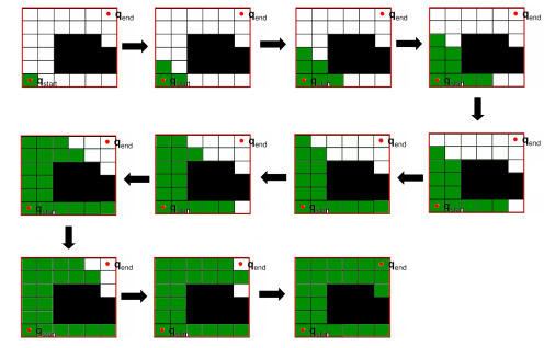
- Begin search at the start node and do a test for goal.
- If start is same as goal, then stop search.
- Otherwise, continue search.
- Visit the adjacent nodes of start and test whether any of them is goal.
- If goal not found, then continue search at the adjacent nodes of the nodes visited in previous step. Skip any node that has already been visited.
- Continue Step 3, until either the goal is found or until all nodes that can be reached from start node have been visited.
Exhaustive or brute-force search strategy
- Enumerate systematically all possible candidates and test if any of them is the goal.
- In breadth-first search, all paths of length ‘n’ from start are
Inplementaion
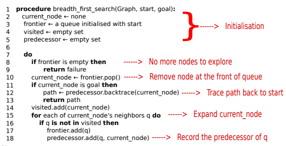
Creates and maintains three lists:
- A list of visited nodes. I These nodes have failed the test for goal node.
- A list of frontier nodes. I Frontier nodes are the neighbours of already visited nodes that have not been visited (goal-tested) yet.
- A list of predecessor nodes. I Predecessor is recorded when a node is expanded, i.e. when its neighbours are added to the frontier list.
Pros
- Simple and easy to implement.
- If a path exists from start to goal, it will always find the shortest path (complete and optimal).
- Suitable for smaller grids (fewer cells).
Cons
Link to original
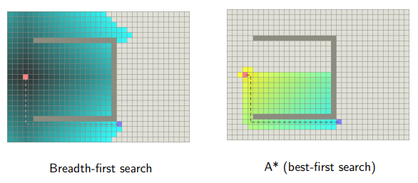
- Searches ‘blindly’. Only adjacency or neighbourhood information is used. (Uninformed search)
- Inefficient, especially for large grids populated sparsely with obstacles.
Informed Search Strategies
Informed Search Strategies
Link to original
- Informed search strategies use knowledge about the problem domain to guide the search more efficiently.
- They evaluate each node using a cost function.
- In path planning problems, the most commonly used cost functions include the estimated distance to the goal node and the actual distance from the start node.
- Informed search strategies are greedy best-first approaches. I Instead of exploring all nodes with equal priority, informed search prioritises the exploration of those nodes that have a lower cost.
Best-First Strategy
A-Star Algorithm
Concept
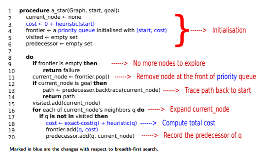
- Heuristic h(q): Estimated length of the path from the node q to the goal node.
- Exact cost g(q): Length of the actual path from the start node to the node q.
- Total cost for node q: f (q) = h(q) + g(q)
Admissible Heuristic
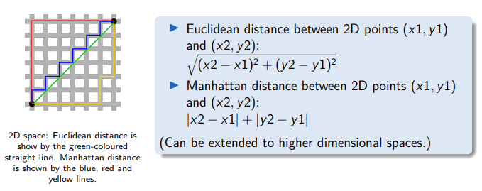
To find an optimal (least-cost) path from start to goal, the heuristic used by A* should be admissible, i.e. it should never overestimate the actual cost of getting to goal node from the current node.
- For a continuous environment (e.g., outdoor feature maps): Euclidean distance, spherical distance, etc.
- For a discrete environment (e.g., indoor occupancy grid maps): Manhattan distance.
Pseudocode
Link to original
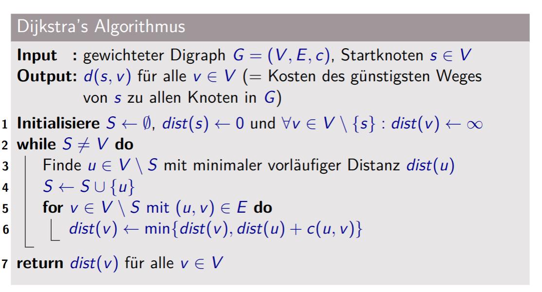
Dijkstra’s Algorithm
Allgemein
- Best-First-Search
- Sehr große Graphen – z.B. Routenplaner
- Bei negative Kantengewichte nicht korrekt! -> Bellmann-Ford Algorithmus
Definition
Laufzeit
Notizen aus RDL
- However, unlike A*, its cost function has only one term, namely the exact cost g(q). This is the actual cost of moving from the start node to node q.
- If the actual cost of moving from a node to an adjacent node is the identical for all nodes in the graph, then Dijkstra’s algorithm is identical to Breadth-First Search.
=> ROS 2 Navigation Stack includes Dijkstra’s and A* path planners.
Link to original

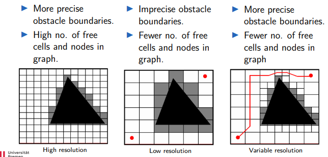
Influence of Grid Map Resolution
Influence of Grid Map Resolution
Link to original
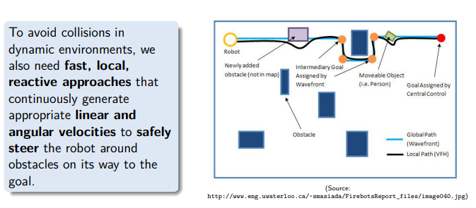
Obstacle Avoidance
Static versus Dynamic Environment
- Path planning finds a globally optimal path to reach the goal pose from the initial pose.
- However, it assumes a static world, i.e. the positions of obstacles are fixed and fully known. I But, real-world environments are dynamic.
- Obstacles may change position dynamically (e.g. furniture may get displaced).
- New obstacles may appear on the scene (e.g. something falls down from the overhead shelf).
- Obstacles may be constantly moving (e.g. people or other robots moving through corridors).
- Global path planning is slow and hence not suitable for fast obstacle avoidance.
Local Approaches
Local Approaches
Basic Idea
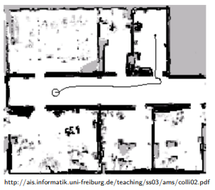
- Sensor data (e.g. lidar, sonar) is used to continuously detect obstacles as the robot moves.
- Odometry data is used to obtain the robot’s current pose and velocity.
- A set of possible solutions (candidates) are generated based on sensor and odometry data to steer the robot.
- An objective function evaluates each possible solution.
- The best (optimal) solution is selected and used to control the robot’s linear and angular velocities.
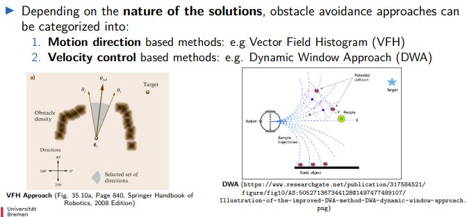
Only a local region around the robot or a short time window is considered at a time for Obstacle Avoidance ==> locally optimal motion control.Categories of Approaches
Link to original
Link to originalDynamic Window Approach
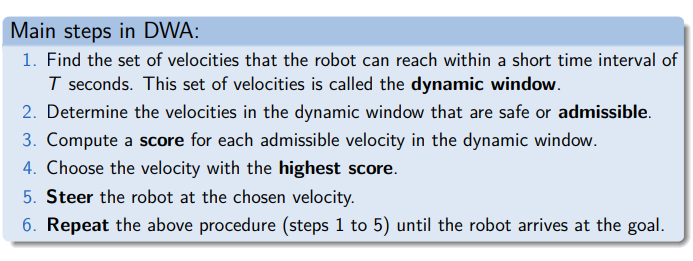
Main Steps
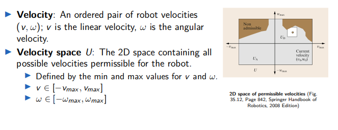
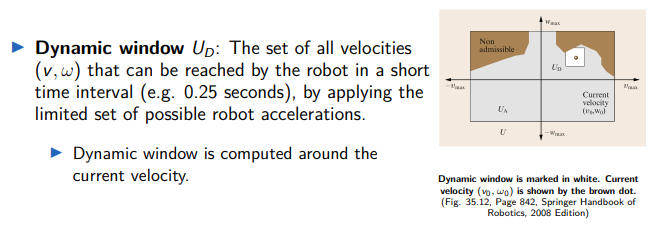
Velocity Space
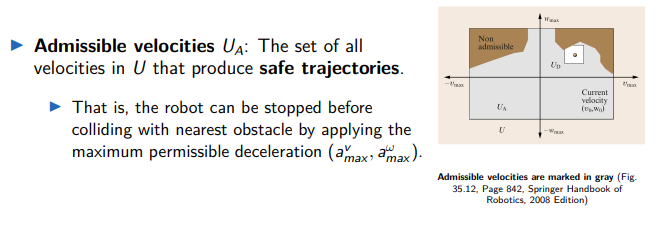
=> Admissible: Grey Area, Non Admissible: Brown Area
=> white BoxObjective function F(v, ω)
The objective function F(v, ω) evaluates trajectories based on three criteria:
- Closeness to goal pose: How close to the goal pose would this trajectory bring the robot?
- Clearance from nearest obstacles: How far is the nearest obstacle on this trajectory?
- Speed of motion: How fast does the robot move on this trajectory? I The objective is to drive in the correct direction as fast as possible while staying as far away from obstacles as possible.
Strengths and Weaknesses
Strength:
Fast approach for Obstacle Avoidance.
Weakness:
Difficulty to enter narrow passages and doorways (robot does not stop on time).
Improved DWA:
Optimize position and velocity simultaneously.
Link to original
ROS 2 Navigation Stack
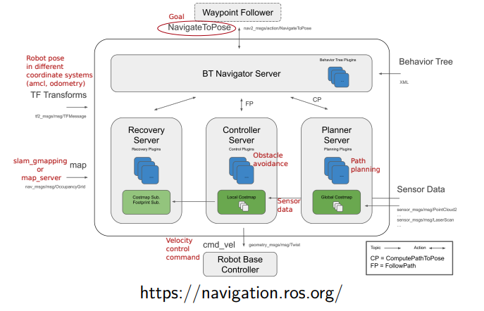
ROS 2 Navigation Stack
Planner Server
Global path planning
A* etcController Server
- Obstical avoidance
Controller Server
- Liniar and Angular Velocity
Behavior Tree
how the robot should react
Link to original
For example: If fails the robot should retry or start recovery strategy
next: RDL VL 08 Task planning